Keeping a two-wheeled robot upright is fundamentally an inverted-pendulum problem: the body (mass M, inertia Jψ) pivots about the wheel axle on an arm of length L = H/2, and the only way to stop its tilt angle ψ from running away is by altering the wheel velocity faster than gravity makes it fall.
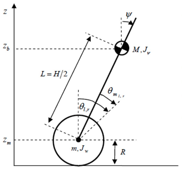
Figure 1: Body tilt ψ, wheel angle θ, and pendulum arm length L = H/2 from the wheel axle up to the body's center of mass.
Getting a usable real-time measurement of ψ (tilt), fundamentally, is the main problem for balance. The accelerometer's Z-axis reading gives a tilt estimate that's accurate but slow and noisy, while integrating the gyro's X-axis rate is fast and responsive but drifts. A Kalman filter fuses the two every 1 ms. The IMU (an MPU-9250) is polled over SPI at that rate, to produce a tilt estimate that counteracts the negative aspects of each sensor, and results in accurate and immediately responsive ψ readings. That filtered tilt, the filtered gyro rate, the average of the two wheel velocities (from the encoders), and the derivative of the gyro rate form a 4-state vector that feeds a full-state feedback law, u = −Kx — the same structure an LQR design produces. In practice: −60 on tilt, −4.5 on gyro rate, −1.1 on wheel velocity, and −0.1 on the gyro-rate derivative — weights that lean hardest on directly countering tilt, with the velocity terms acting as damping so the response doesn't oscillate. The resulting effort is split evenly across both motors, and the whole loop (Kalman filter, state averaging, and the control law) runs at 250 Hz, fast enough to correct a tilt long before the robot falls.
Due to the limited distance the IR sensor can accurately measure, the robot treats ball-finding as an area coverage problem: it follows the field boundary and stops at each corner to scan, and because each corner's scan radius does not reach the center of the field, the robot has to spiral inwards to cover the entire area (see Figure 2). This is achieved by increasing the robot's distance from the wall (the boundary). The moment the ball lands inside a scanned region, the state machine (see Figure 3) breaks out of the search loop and drives straight at it.
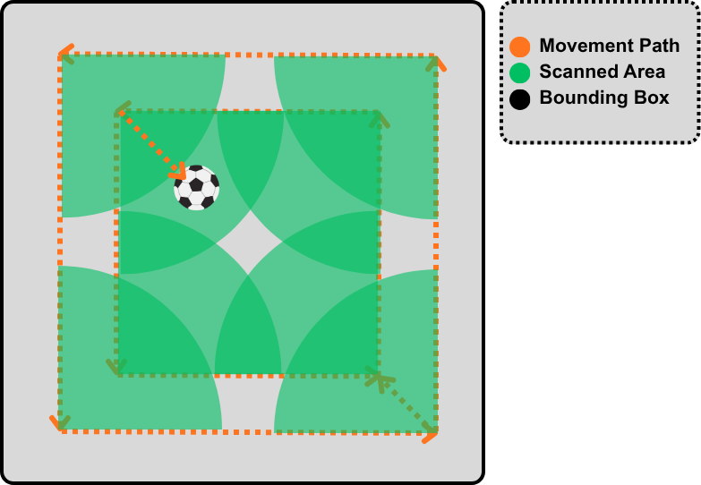
Figure 2: Movement path (orange) and scanned area (green) — four corners cover the whole field with overlap to spare.
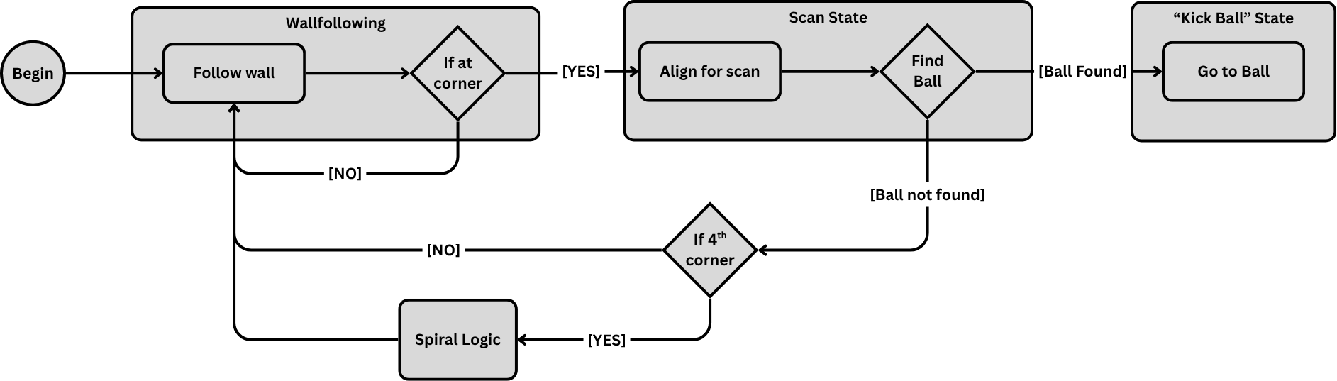
Figure 3: The search finite-state machine: wall-follow → scan each corner → drive to the ball if found, otherwise spiral inward and repeat.
The robot's position reading for this project was calculated using dead reckoning off wheel odometry. This meant any drift in the wheel-speed estimate directly became drift in the robot's position estimate on the field. The finite state machine is built to tolerate that shortcoming: it re-zeros against the field boundary at every corner instead of solely trusting the dead-reckoned position.