LQR vs MPC for Drone Obstacle Avoidance

System Model & Track Geometry

The drone is modeled as a discrete-time 2D double integrator: state x_k = [p_x p_y v_x v_y]^T, input u_k = [a_x a_y]^T, evolving as x_k+1 = Ax_k + Bu_k with sampling time Δt. The track centerline is generated from spline interpolation through anchor points, with inner and outer walls formed by offsetting the centerline by half the track width. Circular obstacles are placed along the track via a signed normal offset from selected centerline indices, with a safety margin keeping the vehicle away from walls and a buffer expanding each obstacle's radius.

       ┌ 1  0  Δt  0 ┐            ┌ ½Δt²   0  ┐
   A = │ 0  1  0  Δt │        B = │  0   ½Δt² │
       │ 0  0  1   0 │            │  Δt    0  │
       └ 0  0  0   1 ┘            └  0    Δt  ┘

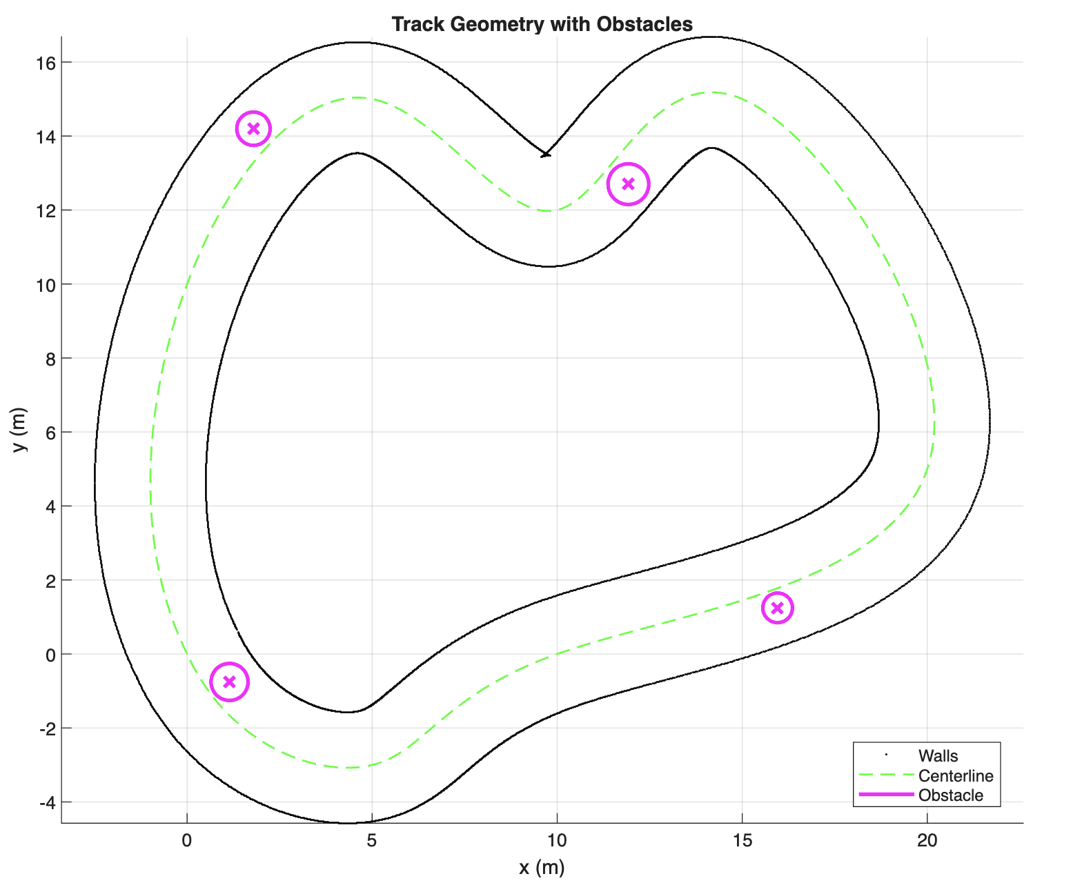
Fig. 1 — track geometry: spline-generated centerline, inner/outer walls, and the four circular obstacles both controllers had to avoid.

Reactive Control: LQR + Potential Fields

The LQR controller minimizes a quadratic cost with weights Q ≥ 0 and R > 0, producing a feedback gain K and the tracking law u_LQR = −K(x − x_ref), where x_ref is a lookahead target advanced along the centerline each step. Walls and obstacles separately generate a repulsive acceleration term based on distance-to-obstacle — optionally including a damping term and a tangential "vortex" component to help the vehicle slide past rather than stall — and the two terms are summed and saturated to the actuator limits: u = sat(u_LQR + u_pot). This is computationally light enough to run on embedded hardware, but because the repulsive field is nonconvex, it can introduce local equilibria that the tracking term alone can't escape.

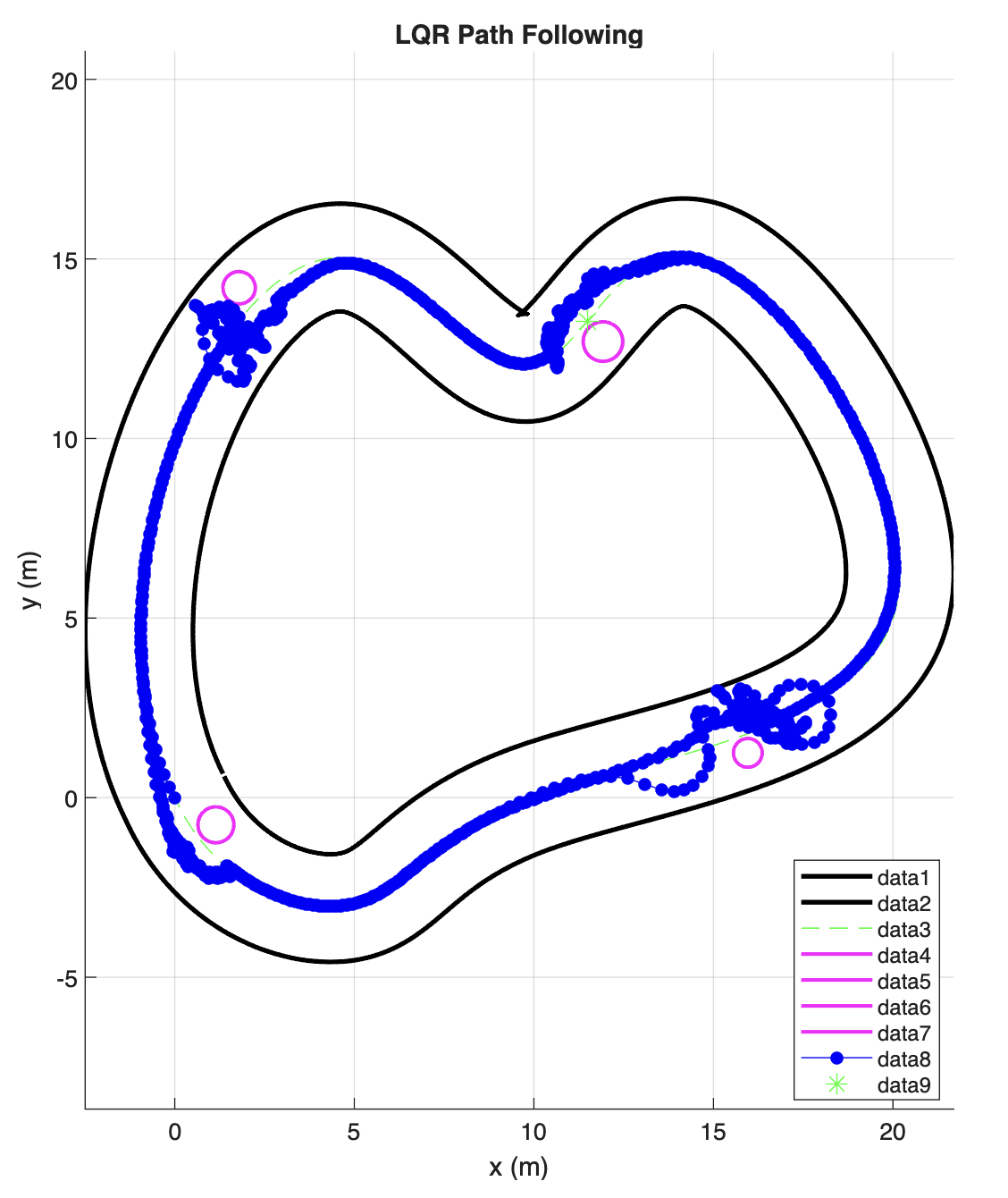
Fig. 2 — LQR + potential-field trajectory. The drone gets caught oscillating near three of the four obstacles, reaching only 16.33% of the lap.

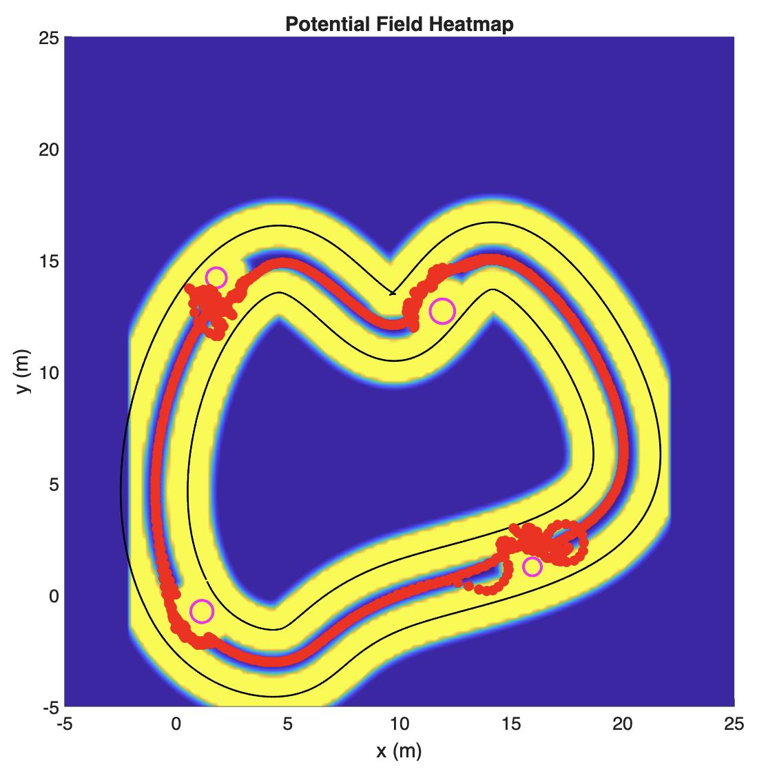
Fig. 3 — the potential field driving Fig. 2's repulsion. The red trajectory visibly tangles right where the field's gradients are steepest and least convex.

Predictive Control: Constrained MPC

At each step, MPC solves a finite-horizon optimal control problem over horizon N, choosing the control sequence that minimizes tracking error and control effort subject to the drone's own dynamics:

min Σ ‖x_i − x_i^ref‖²_Q + ‖u_i−1‖²_R

subject to actuator bounds ‖u_k‖_∞ ≤ u_max, a "track-tube" constraint limiting deviation from the centerline, and obstacle-avoidance constraints requiring distance from each obstacle center to exceed its buffered radius. Only the first optimal input is applied, the horizon shifts forward, and the problem is re-solved at the next step, warm-started from the previous solution. Because it explicitly plans ahead under these constraints instead of only reacting when close, MPC anticipates upcoming curvature and obstacles — at the cost of solving a constrained optimization in real time on every step.

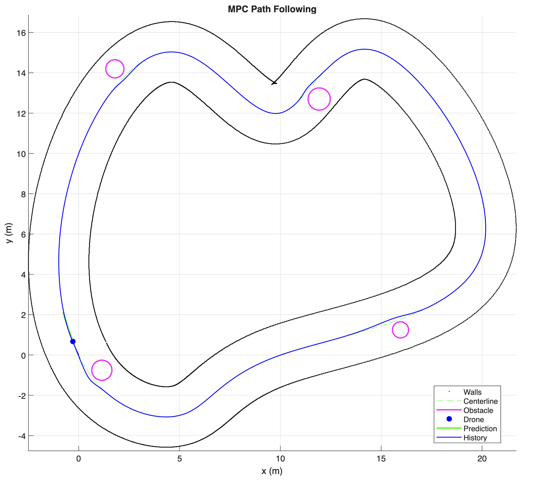
Fig. 4 — MPC trajectory: one smooth pass around the full track (117.08% of the lap — it completed the loop and kept going), with clean avoidance at every obstacle.

Theory: Why Each Controller Applies

Both approaches are backed by more than simulation plots. Controllability is established first: for any Δt > 0, the (A, B) pair decouples into two identical 1D subsystems, each with a controllability matrix whose determinant works out to exactly −Δt³ — nonzero for any real timestep, so the system is controllable regardless of how the simulation is tuned. Given that, the discrete-time algebraic Riccati equation is shown to admit a unique stabilizing solution P ≥ 0, whose corresponding feedback gain K places every eigenvalue of the closed-loop matrix A − BK strictly inside the unit circle — closed-loop stability, not just an empirically-tuned gain. For a moving lookahead reference with bounded increments, this stability argument extends to input-to-state stability, giving a tracking-error bound proportional to how fast the reference moves. Those guarantees, however, apply only to the linear LQR portion — saturation and the nonlinear potential-field term can invalidate them globally, which is exactly what shows up in simulation as the oscillation and local-minima behavior in Fig. 2.

For MPC, a separate proposition shows that if the constrained optimization is feasible at a given step and solved to a solution, applying only its first control input guarantees the next actual state satisfies every constraint used in that optimization — because the plant is simulated with the exact same dynamics the optimizer assumed. A further proposition notes that with linear dynamics and a quadratic cost, MPC would reduce to a quadratic program if the constraint set were linear — but here the distance-based track and obstacle constraints are nonlinear and nonconvex, so the controller is really solving a nonlinear program each step, locally solvable in real time for a moderate horizon but not immune to infeasibility or poor convergence.

Quantitative Results

Both controllers ran on the identical spline-generated track and obstacle layout. Neither ever violated a wall constraint, but beyond that baseline safety requirement, the two approaches diverged sharply:

Metric                           LQR+PF      MPC
Progress (% of lap)               16.33     117.08
Wall violations (any)             False      False
Wall violation fraction           0.000      0.000
Minimum obstacle clearance (m)    0.873      0.250
RMS cross-track error (m)         0.107      0.031
Max cross-track error (m)         0.158      0.153
u_RMS (m/s²)                      8.376      0.219
Δu_RMS (m/s²)                    13.908      0.058
MPC solve time mean (s)               –      0.066
MPC solve time max (s)                –      0.235

MPC cut RMS cross-track error by roughly 3.5× (0.107 m → 0.031 m) while requiring nearly 40× less control effort (u_RMS 8.376 → 0.219 m/s²) and far smoother commands (Δu_RMS 13.908 → 0.058 m/s²) — the numeric signature of the oscillation visible in Fig. 2. LQR+PF was actually more conservative around obstacles (0.873 m minimum clearance vs. MPC's 0.250 m), but that conservatism is exactly what cost it forward progress: it covered only 16.33% of the lap before the simulation ended, against MPC's 117.08% (a full lap, and then some). MPC's own cost is computational: a mean solve time of 0.066 s comfortably fits the 0.1 s sampling period, but its worst case — 0.235 s — exceeds the real-time deadline outright, a real, measured limitation rather than a hypothetical one.

Neither limitation is a surprise given the theory above: LQR's guarantees never covered the nonlinear, saturated closed-loop system it was actually running in, so the limit-cycle behavior near obstacles is expected, not a tuning failure. And MPC's obstacle constraint is a nonconvex distance-to-circle condition, so the nonlinear program it solves each step can occasionally take meaningfully longer near cluttered regions — precisely where the worst-case solve time shows up. Future work identified directly from this gap: replacing the point-distance obstacle constraints with continuous signed-distance geometry, and adding explicit Δu penalties to the cost to smooth control effort further without relying on tuning alone.