3-DOF Robot Arm Simulator

A 3-degree-of-freedom robot arm, simulated entirely on an FPGA board and rendered live in an isometric 3D view over HDMI at 60 FPS — driven by a USB keyboard, solved with an from-scratch inverse-kinematics solver, and wrapped in a pick-and-place game with a live score.

System Architecture

The system splits cleanly into two halves that talk over AXI: a MicroBlaze soft-core processor handling USB input, target tracking, inverse kinematics, and the pick-and-place game logic in C, and a SystemVerilog hardware pipeline handling the register file, CORDIC math, isometric projection, and the HDMI signal itself. Every piece of live state — joint angles, target and object positions, score, and game state — is written one-directionally from the MicroBlaze into an AXI4-Lite register file, which the hardware side reads and never writes back to.

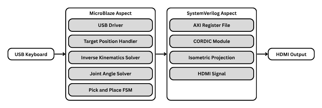
Datapath diagram showing USB Keyboard feeding into a MicroBlaze aspect (USB Driver, Target Position Handler, Inverse Kinematics Solver, Joint Angle Solver, Pick and Place FSM), which feeds into a SystemVerilog aspect (AXI Register File, CORDIC Module, Isometric Projection, HDMI Signal), which outputs to HDMI.

Fig. 1 — full datapath: USB input → MicroBlaze software pipeline → AXI register file → SystemVerilog hardware pipeline → HDMI output.

Offset  Register    Description
0x00    Theta1      Shoulder Yaw Angle
0x04    Theta2      Shoulder Pitch Angle
0x08    Theta3      Elbow Pitch Angle
0x0C    Target_X    End Effector Target X
0x10    Target_Y    End Effector Target Y
0x14    Target_Z    End Effector Target Z
0x18    Obj_X       Object X Position
0x1C    Obj_Y       Object Y Position
0x20    Obj_Z       Object Z Position
0x24    Score       Score Value
0x28    State       Pick and Place State

The AXI4-Lite register file — the entire hardware/software interface, 11 registers wide.

The Vivado block design underneath ties the MicroBlaze, its AXI interconnect, the UART and USB peripherals, and the custom HDMI controller IP together — the actual hardware described above lives inside that hdmi_text_controller_0 block.

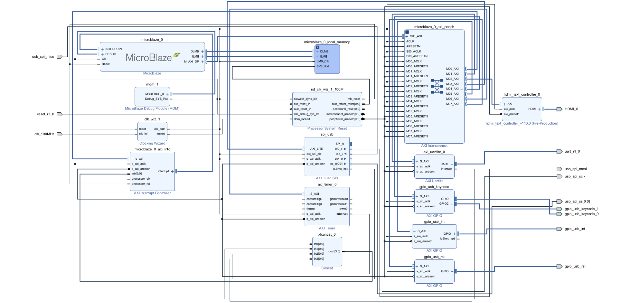
Vivado block design diagram showing the MicroBlaze processor, AXI interconnect, clocking and reset IP, USB and UART peripherals, and the custom HDMI controller IP, all wired together via AXI.

Fig. 3 — the full Vivado block design: MicroBlaze, AXI interconnect, peripheral IP, and the custom HDMI controller.

Isometric Rendering Pipeline

The hardware renders a true 3D world in a 2D isometric view using a fixed 30° camera transform. Given a 3D point (x, y, z), the transform to 2D screen coordinates is:

x_display = (x − z) · cos(30°)
y_display = −y + (x + z) · sin(30°)

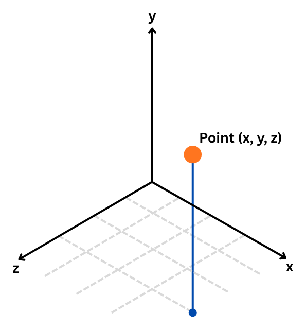
Isometric view diagram showing a 3D axis (x, y, z) with a point plotted above the ground plane, illustrating the coordinate transform used for the rendering pipeline.

Fig. 2 — the isometric coordinate transform this rendering pipeline is built on.

Those screen coordinates are computed downstream of the CORDIC module, which supplies the sine and cosine of each joint angle needed to turn a joint angle into a 3D vector in the first place. Four pairs of screen coordinates come out the other end of the pipeline — base, shoulder, elbow, and end effector — which the renderer connects with three 2-pixel-wide line segments (base→shoulder, shoulder→elbow, elbow→end effector), extending the line-drawing logic built for pixel drawing in an earlier lab. A pixel is colored in if it falls within a 2-pixel Manhattan distance of any active segment, which is what keeps the arm links solid and gap-free. The actual rendered output is shown at the top of this page.

CORDIC Trigonometric Unit

SystemVerilog has no native trigonometric functions, so sine, cosine, and atan2 — all required for the isometric transform and the inverse kinematics — are computed by a custom CORDIC (COordinate Rotation DIgital Computer) module: a shift-and-add algorithm that approximates a rotation through a sequence of small, predefined angle steps using only a precomputed atan lookup table, with no floating-point hardware anywhere in the design. The module runs in two modes — rotation (given a vector and an angle, rotate it) and vectoring (given a vector, find its angle) — each converging over 16 add-shift iterations.

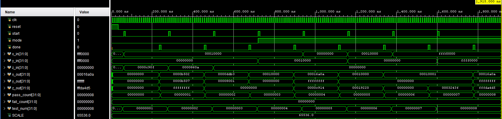
Simulation waveform of the CORDIC module showing clk, reset, start, mode, and done signals along with x_in, y_in, z_in, x_out, y_out, z_out, and pass/fail counters across 8 test cases.

Fig. 7 — simulation waveform covering all 8 CORDIC test cases, rotation and vectoring mode.

Test  Mode       Input           Output
1     Rotation   (1,0) by π/4    cos/sin = 0.707 / 0.707
2     Rotation   (1,0) by π/6    cos/sin = 0.866 / 0.500
3     Rotation   (1,0) by 0      1.0 / 0.0 (unchanged)
4     Vectoring  atan2(1, 1)     π/4  = 0.785 rad
5     Vectoring  atan2(1, 0)     π/2  = 1.571 rad
6     Vectoring  atan2(0, 1)     0 rad
7     Vectoring  atan2(0, -1)    π    = 3.142 rad
8     Vectoring  atan2(-1, -1)   -3π/4 = -2.356 rad

All 8 simulated test cases matched their expected outputs exactly.

Inverse Kinematics & Motion

Rather than solve the full 3-DOF problem at once, the IK solver decomposes it into a 1-DOF shoulder yaw rotation followed by a 2-DOF planar problem in the vertical plane containing the target: yaw comes directly from the ground-plane projection of the target, and the shoulder pitch and elbow pitch are solved from the law of cosines.

// shoulder yaw
theta[0] = atan2f(target.y, target.x);

float r = sqrtf(target.x * target.x + target.y * target.y);
float h = target.z - shoulder_height;
float D = (r * r + h * h - L1 * L1 - L2 * L2) / (2.0f * L1 * L2);
D = clampf(D, -1.0f, 1.0f);

// elbow pitch
theta[2] = atan2f(-sqrtf(1.0f - D*D), D);

// elbow-down
theta[1] = atan2f(h, r) - atan2f(L2 * sinf(theta[2]), L1 + L2 * cosf(theta[2]));

The full inverse-kinematics solve, in C, running on the MicroBlaze.

A target position handler sits in front of the solver: it reads USB keycodes (w/a/s/d for the X-Y plane, e/q for Z) and applies a signed 0.05-unit delta to the current end-effector target along the corresponding axis, clamped to the arm's feasible range of motion. Rather than writing the IK solution straight to the register file — which would make the arm snap instantly to each new target — a joint angle interpolator moves each joint toward its solved target by a bounded step every frame, which is what makes the arm's motion read as continuous and smooth instead of jumpy.

Pick-and-Place Game Logic

On top of the arm and IK stack sits a 6-state finite state machine — IDLE, APPROACH PICK, PICK, APPROACH PLACE, PLACE, SCORE — that turns the simulator into an actual game. The first three states are gated on the distance from the end effector to the object; the last three are gated on the distance from the object to the target drop-off position. Crossing a pick-radius threshold advances the state, and completing a full pick-and-place cycle increments the score and loops back to start a new round.

Finite state machine diagram: IDLE leads to Approach Pick, which leads to Pick when distance is less than the pick radius, then Approach Place, then Place when distance is less than the pick radius, then Score, which loops back to Approach Pick for a new round.

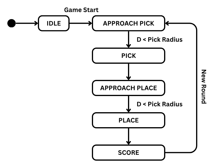
Fig. 6 — the 6-state pick-and-place finite state machine.

In the final demo, the full loop worked end to end: the arm solved its own inverse kinematics correctly in 3D space, rendered that motion live over HDMI in isometric view, and the pick-and-place FSM correctly tracked an object from pickup through placement and scored it. Two things were genuinely harder than expected: Vivado repeatedly synthesized against a cached, stale version of the custom IP instead of the latest edits, so bug fixes silently failed to show up in hardware until the cache issue was tracked down — a persistent annoyance through most of development — and wiring the USB keyboard into the rest of the datapath took more effort than the earlier labs it was adapted from suggested it would.