Differential Drive Robot — Full Autonomy Stack

Final project, ME 498: Robotic Software Engineering — Group 1, University of Illinois Urbana-Champaign. Team of 7.

A complete three-layer autonomous navigation stack for a planar differential-drive robot: A* search finds a globally optimal path through a cluttered 2D environment, a Timed Elastic Band optimizer time-parametrizes and smooths it, and a clamped cubic spline turns the result into a continuous reference that a modified PI controller tracks in closed loop — plus receding-horizon dynamic-obstacle avoidance and multi-target trajectory chaining as extensions.

Technical Highlights

A* on an inflated occupancy grid — an 8-connected best-first search on a 0.1 m grid finds a 3.653 m collision-free path (170 nodes expanded); an optional soft-cost inflation layer trades a 3.2% longer path for a guaranteed 0.2 m clearance from every obstacle.
Timed Elastic Band optimization — a six-term nonlinear cost (time, smoothness, obstacle clearance, kinematic limits, boundary rest, and acceleration smoothing) reshapes the discrete A* path into a time-parametrized trajectory with a smooth trapezoidal speed profile instead of a bang-bang one.
Receding-horizon dynamic obstacle avoidance — replanning every 0.2 s over a 1 s horizon against a moving sinusoidal obstacle, holding minimum clearance at 0.250 m against a 0.150 m safety floor across 94 replanning cycles with zero violations.
C² cubic spline tracking — clamped cubic splines turn the discrete TEB waypoints into a twice-differentiable reference, tracked by a PI controller with five targeted body-frame fixes (signed velocity, folded heading error, a velocity cap, a lower outer-loop gain, and a heading deadband) to eliminate spin-out and noise-driven oscillation.
Multi-target trajectory chaining — three sequential A* → TEB → spline segments joined with C¹ continuity at each intermediate target, completing a 30.2 s multi-leg mission with 0.087 m terminal error.
Tested against an existing simulator — the planner integrates with the team's existing estimation/control simulator (built in earlier course midterms) purely through duck-typed interfaces, with no upstream modification, backed by 151 passing tests.

Global Path Planning — A*

The workspace is a planar differential-drive robot (mass 2 kg, radius 0.2 m, track width 0.15 m) navigating a 2D grid with two large rectangular obstacles, from a start at (−1.2, −1.3) to a goal at (1.2, 1.3). An A* best-first search on a 0.1 m occupancy grid, using an 8-connected motion set and an admissible Euclidean-distance heuristic, finds a globally optimal collision-free route: 170 nodes expanded, 3.653 m path length. Because the plain search hugs obstacle corners with zero safety margin, an optional inflation layer marks cells within the robot's own radius of any obstacle as soft-cost zones — traversable, but penalized — which routes the path through the center of wide corridors while still permitting narrow passages that a hard inflation would block outright. The cost: a 3.770 m path, +3.2% longer, in exchange for a guaranteed 0.2 m clearance from every obstacle edge.

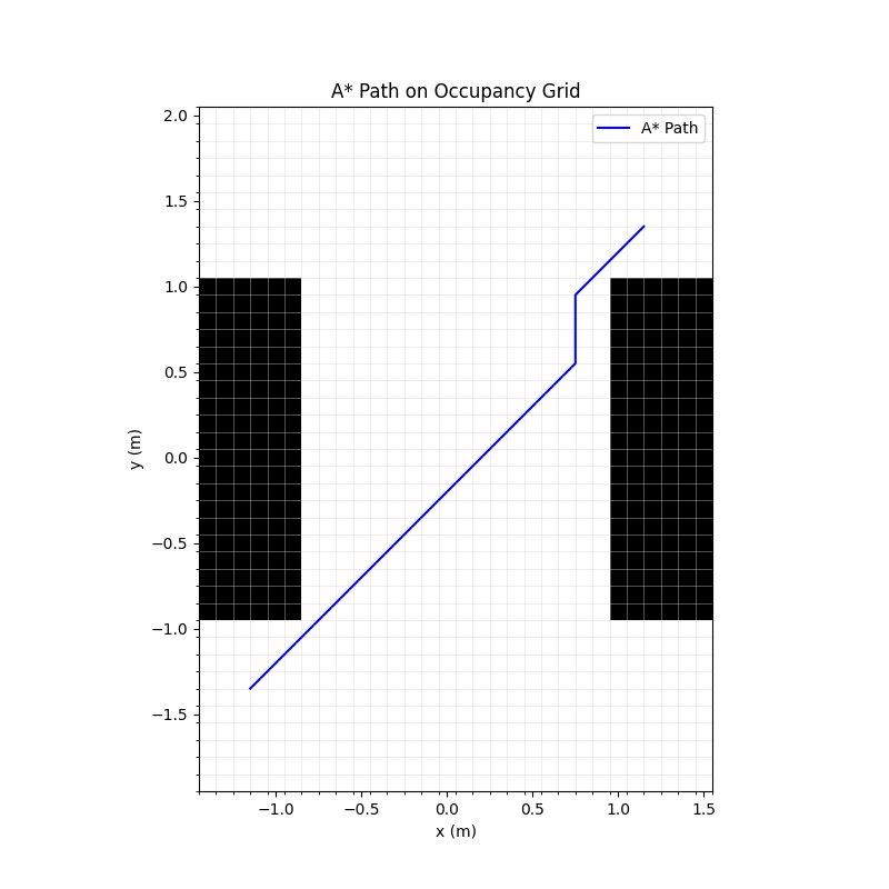
A* planned path overlaid on the occupancy grid, showing a diagonal route between two black rectangular obstacles from bottom-left to top-right.

Fig. 2 — plain A* path (3.653 m), hugging the inner obstacle corner.

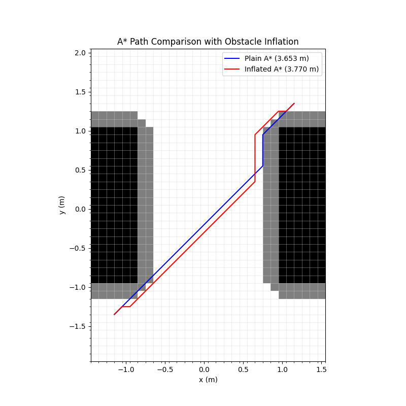
Comparison of the plain and obstacle-inflated A* paths, with the inflated path detouring around a gray soft-cost buffer zone surrounding each obstacle.

Fig. 3 — plain (blue, 3.653 m) vs. inflated (red, 3.770 m) A* paths.

Trajectory Refinement — Timed Elastic Band

The A* path is globally correct but kinematically crude — no timing information, sharp turns, no respect for the robot's speed limit. A Timed Elastic Band (TEB) optimizer refines it into a trajectory of waypoint positions and time intervals, warm-started from the A* path and solved with L-BFGS-B, by minimizing a six-term composite cost:

J = γ_timeΣ Δt + γ_smoothΣ‖Δx‖² + γ_obsΣ max(d_min−d, 0)²
+ γ_velΣ max(v̄−v̄_max, 0)² + γ_bc(v̄₀² + v̄_N−1²) + γ_accΣ(v̄_k+1−v̄_k)²

Each term does a distinct job: time favors fast traversal, smoothness keeps the path compact, obstacle clearance repels waypoints from obstacles, velocity and boundary terms enforce kinematic and rest-to-rest constraints, and the acceleration term — added on top of the base formulation — penalizes speed changes between adjacent segments. That last term is what turns a bang-bang velocity profile into a smooth trapezoidal ramp: roughly 2.5 s to reach the 0.5 m/s speed limit, a 4 s cruise, and a 2 s ramp to rest, for a total mission time of 8.471 s — 17% slower than the unregularized version, a deliberate trade of speed for actuator-friendly motion. The solver didn't fully converge within its 200-iteration budget, but a hard post-solve projection guarantees the output still satisfies every speed and clearance constraint regardless.

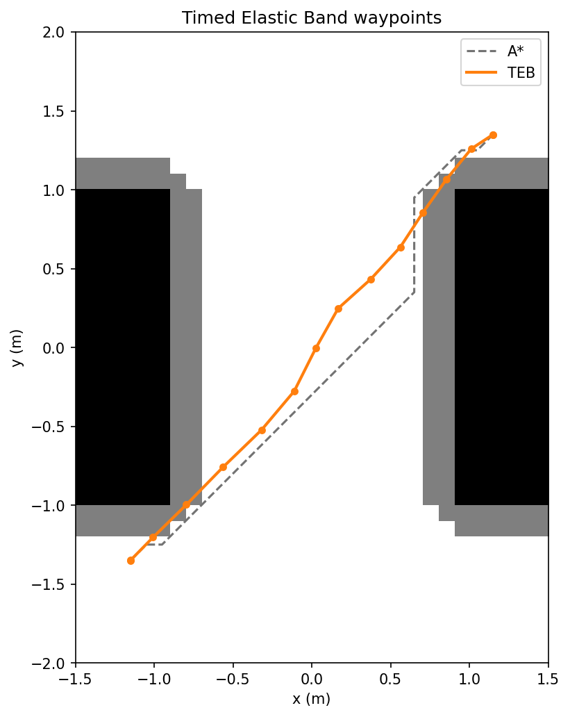
TEB-optimized waypoints overlaid on the original A* path, pulling the trajectory into a smoother diagonal away from the obstacle edges.

Fig. 4a — TEB waypoints (orange) vs. the original A* path (gray dashed).

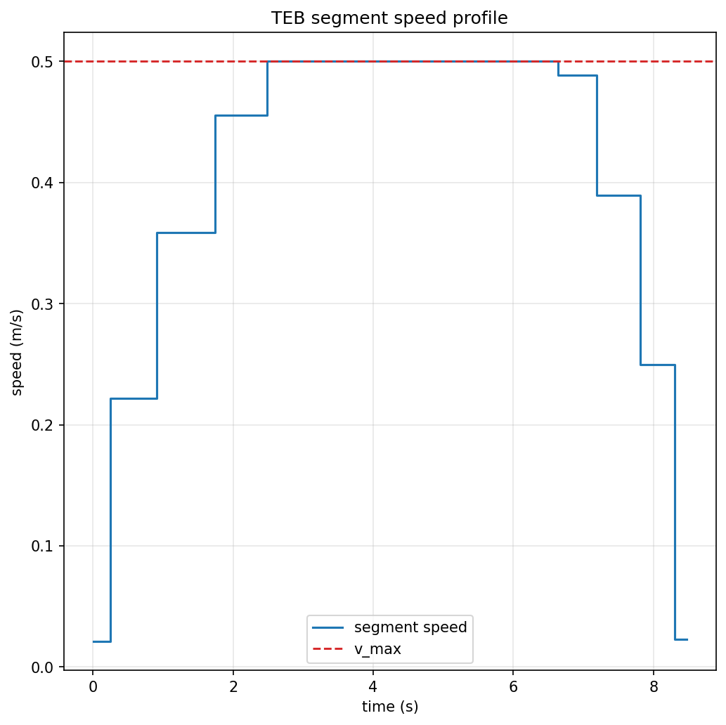
Fig. 4b — resulting speed profile: a smooth trapezoidal ramp, not bang-bang.

Dynamic Obstacle Avoidance

A receding-horizon extension of the same TEB optimizer handles moving obstacles: it replans every 0.2 s over a short 1 s window, warm-started from the previous plan, evaluating clearance against the obstacle's predicted position rather than a fixed one. Tested against a sinusoidal obstacle sweeping across the corridor, the planner ran 94 replanning cycles over an 18.6 s mission and never dropped below 0.250 m of clearance — comfortably above the 0.150 m safety floor, with zero violations. That margin is deliberate: the planning target is set above the reporting floor because the underlying soft penalty has zero gradient once a constraint is already satisfied, so without that headroom the optimizer has no signal left to push it away from the boundary.

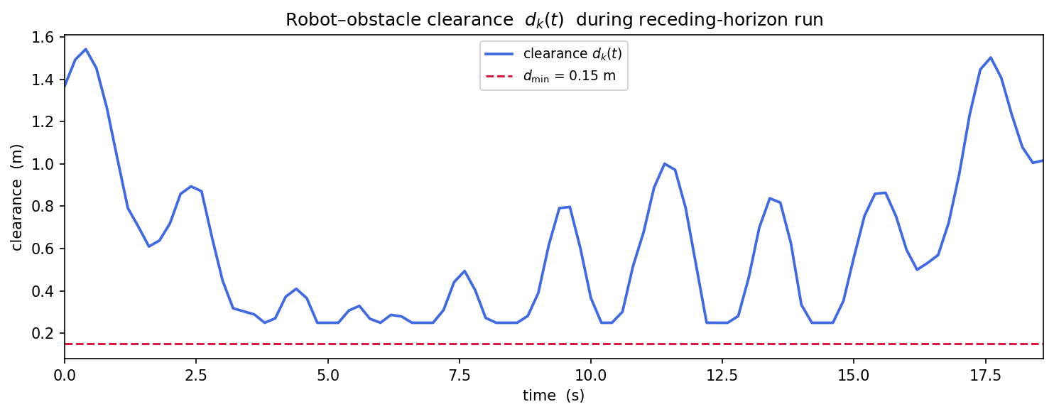
Robot-obstacle clearance over time during the receding-horizon run, oscillating between roughly 0.25 and 1.55 meters and never approaching the 0.15 meter safety floor.

Fig. 5 — robot–obstacle clearance over the full receding-horizon run; the trace never approaches the 0.15 m floor (dashed red).

Reference Tracking — Cubic Spline + PI Control

Piecewise-linear interpolation between TEB waypoints would introduce velocity kinks and impulsive actuator commands, so a clamped cubic spline fits a C²-continuous reference through them instead — smooth position, velocity, and acceleration everywhere, with zero-velocity boundary conditions at the start and goal. The existing PI controller tracks this reference without any architectural changes, but five targeted edits to its body-frame projection were necessary for stable tracking: using the signed forward-velocity command instead of its magnitude (so the robot can brake or reverse on overshoot instead of always pushing forward), folding the heading error into the body frame so a target behind the robot triggers a reverse rather than a 180° spin, hard-capping the reference speed at the 0.5 m/s limit, lowering the outer position gain so the feedforward velocity dominates instead of cutting corners, and a heading deadband below 0.05 m/s to kill noise-driven oscillation at the held goal. The result tracked the spline reference to a terminal error of 0.0154 m — well inside the one-robot-radius (0.2 m) criterion — with wheel forces saturating only briefly through the tightest corner.

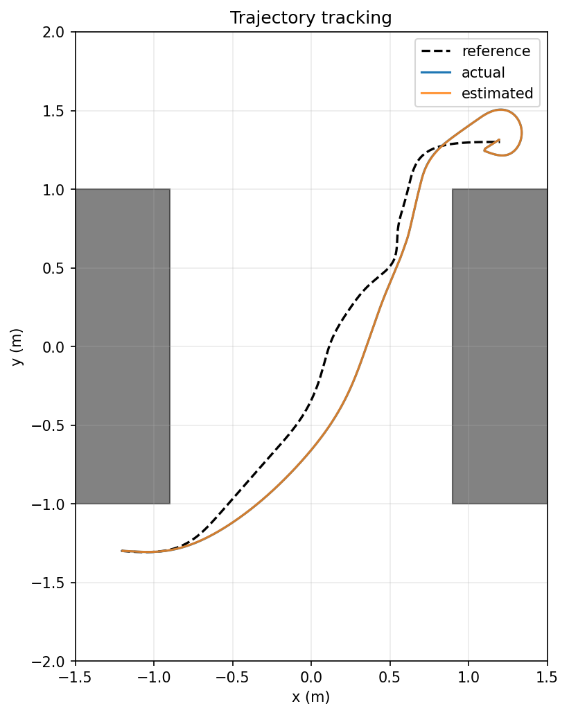
2D trajectory plot showing the spline reference as a dashed S-curve and the actual/estimated robot path closely following it through the corridor to the goal.

Fig. 6a — closed-loop tracking of the cubic-spline reference (dashed) through the corridor.

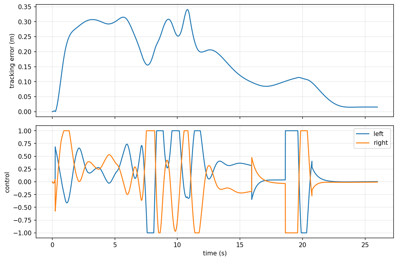
Tracking error over time, peaking around 0.34 meters during the corridor turn and decaying to about 0.015 meters at the held goal, with left and right wheel control commands shown below.

Fig. 6b — tracking error (top) and per-wheel control commands (bottom); error peaks mid-corner, then decays to 0.015 m at rest.

Multi-Target Trajectory Chaining

The same A* → TEB → spline pipeline chains across multiple sequential targets: three randomly generated goal points, C¹ continuity enforced at each intermediate target by matching first derivatives across adjacent spline segments, and a wider 0.35 m planning clearance to give the closed-loop controller more headroom through tighter turns. The full three-leg, 30.247 s mission reached all three targets with a 0.373 m moving-window RMSE, a 0.767 m peak error at the sharpest transition, and a 0.087 m terminal error after the hold phase. Actuator saturation occurred on 16% of timesteps, concentrated at target transitions; the tightest turn's footprint clearance dipped to about −3 mm — a hairline overlap against a reference that itself only budgeted 10 cm of clearance there, not a planning failure so much as the closed-loop tracking having essentially no margin left to give at that specific corner.

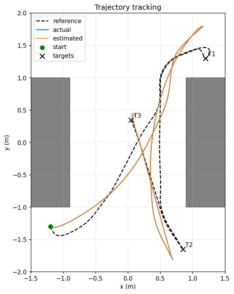
2D plot of the multi-target mission showing the robot visiting three target points in sequence around both obstacles, with the actual path closely tracking the planned reference.

Fig. 7 — multi-target reference (dashed) and closed-loop tracking (orange) across all three targets.

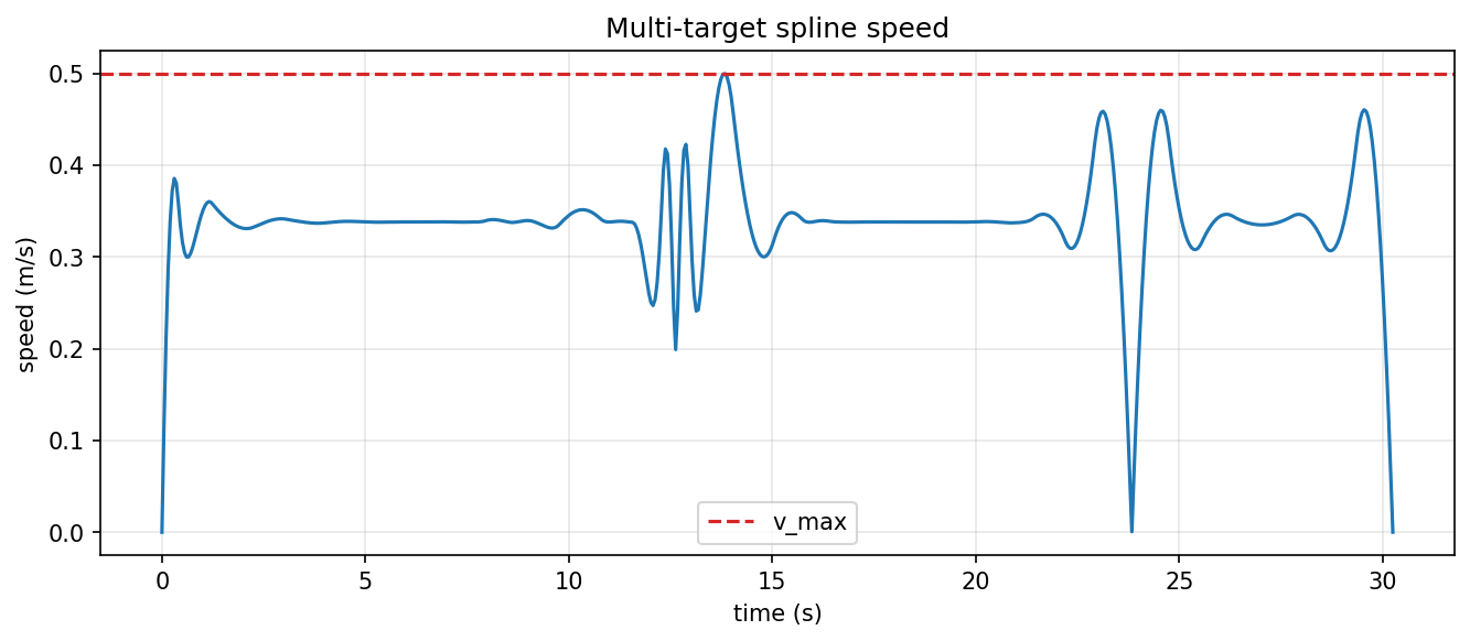
Fig. 7b — speed across the three-leg mission, dipping and spiking at each segment transition.

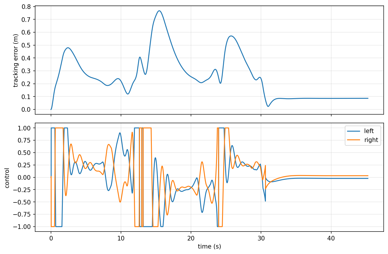
Tracking error across the multi-target mission peaking near 0.77 meters at the sharpest turn, settling to about 0.09 meters, with left and right wheel control commands shown below.

Fig. 8 — tracking error (top) and control effort (bottom) across the full multi-target mission; error peaks at segment transitions, then settles.

A few limitations are called out directly in the team's own report rather than glossed over: the TEB solver didn't reach numerical convergence within its 200-iteration budget on the base task (the post-solve projection still guarantees feasibility, just not necessarily the smoothest possible plan); the dynamic-obstacle extension evaluates against a known, deterministic obstacle trajectory rather than a sensor-driven prediction; and the closed-loop controller saturates its actuators through the tightest corners because the per-wheel force budget is tight relative to the cornering demand at the specification's 0.5 m/s speed limit. None of these blocked the mission from completing — they're the team's own list of what a next iteration would tighten up.